ScaleupROM
This page provides a list of ScaleupROM example applications. ScaleupROM is a projection-based reduced order model code with discontinuous Galerkin domain decomposition (DG-DD) using libROM and MFEM. It aims to create a robust and efficient large-scale ROM that is trained only from small scale component samples which can be used to solve a variety of physics PDEs. For more information, refer to the ScaleupROM repo and online wiki.
Select from the categories below to display examples that contain the respective feature. All examples support (arbitrarily) high-order meshes and finite element spaces. The numerical results from the example codes can be visualized using the GLVis or VisIt visualization tools. See the GLVis and VisIt websites for more details.
Application (PDE)
Reduced order model type
Assembly
Hyper-reduction
Physics code
Stokes flow
This example demonstrates the use of ScaleupROM to create a reduced order model for the Stokes flow problem discretized using Taylor-Hood elements. The governing equation for Stokes flow is defined as $$ - \nu \nabla^2 \mathbf{\tilde{u}} + \nabla \mathit{\widetilde{p}} = 0 $$
$$ \nabla \cdot \mathbf{\tilde{u}} = 0 $$
with boundary conditions
$$ \mathbf{\tilde{u}} = \mathbf{g}_{di} $$
$$ \mathbf{n} \cdot ( - \nu \nabla \mathbf{\tilde{u}} + \mathit{\widetilde{p}} \mathbf{I}) = \mathbf{g}_{ne} $$
where $\mathbf{u}$ and $p$ denote the velocity and pressure field respectively, and $\nu \equiv \frac{\mu}{\mu_0} = 1.1$ is the non-dimensionalized dynamic viscosity with respect to a reference value.
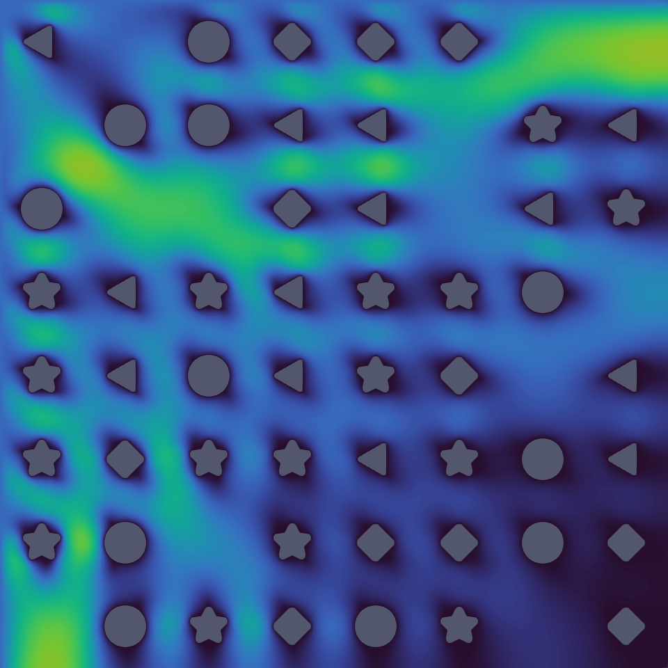
The global-scale system is constructed using a random arrangement from five different reference components: empty, circle, triangle, square, and star. In this example, the fluid flows past an array of these components. Sample snapshots for basis training are generated on 2x2 component domains to better capture downstream flow. A total of 1400 sample snapshots were taken for this example.
On each sample domain, the inflow velocity Dirichlet boundary condition is parameterized as
$$ \mathbf{g}_{di} = (g_1 + \Delta g_1 \sin 2\pi (\mathbf{k}_1 \cdot x + \theta_1),\ g_2 + \Delta g_2 \sin 2\pi (\mathbf{k}_2 \cdot x + \theta_2)) $$
where the parameters are chosen from a uniform random distribution,
$$ g_1, g_2 \sim U[-1, 1] $$
$$ \Delta g_1, \Delta g_2 \sim U[-0.1, 0.1] $$
$$ \mathbf{k}_1, \mathbf{k}_2 \sim U[-0.5, 0.5]^2 $$
$$ \theta_1, \theta_2 \sim U[0, 1] $$
Boundaries at the surface of the object inside the domain have a no-slip wall boundary $g_{di} = 0$ and boundaries on interior interfaces have a homogeneous Neumann boundary $g_{ne} = 0$.
The figure above shows the ROM prediction for $\mathbf{u}$ on a 8x8 system composed of random components with parameter values $g_1 = 1.5, g_2 = -0.8, \Delta g_1 = \Delta g_2 = 0$.
One can follow the command line options below to reproduce the numerical results summarized in the table below:
Generate Meshes:
cd build/examples/stokes
mkdir snapshots basis paraview rom-system
./setup_stokes.sh
- Sample Generation:
../../bin/main -i stokes.sampling.yml - ROM Training:
../../bin/main -i stokes.sampling.yml -f main/mode=train_rom - ROM Building:
../../bin/main -i stokes.sampling.yml -f main/mode=build_rom:main/use_rom=true - ROM Prediction:
../../bin/main -i array.8.yml
The table below shows the ROM performance for the 8x8 system.
| FOM Solution time | ROM Solution time | Speed-up | $\mathbf{u}$ relative error | $p$ relative error |
|---|---|---|---|---|
| 0.08298 sec | 0.00408 sec | 20.34 | 4.193e-3 | 3.030e-3 |
The code that generates the numerical results above can be found in (stokes_flow)
