This page provides a list of libROM example applications. For detailed
documentation of the libROM sources, including the examples, see the online
Doxygen documentation or the
doc directory in the distribution. The goal of the example codes is to
provide a step-by-step introduction to libROM in simple model settings.
Select from the categories below to display examples and miniapps that contain
the respective feature. All examples support (arbitrarily) high-order meshes
and finite element spaces. The numerical results from the example codes can
be visualized using the GLVis or VisIt visualization tools. See the GLVis
and VisIt
websites for more details.
Users are encouraged to submit any example codes and miniapps that they have
created and would like to share. Contact a member of the libROM team to report
bugs
or post questions
or comments.
**Application (PDE)**
**Reduced order models type**
**Parameterization type**
**hyper-reduction**
**Physics code**
**Optimization solver**
Global pROM for Poisson problem
This example code demonstrates the use of libROM and MFEM to define a reduced
order model for a simple isoparametric finite element discretization of the
Poisson problem
$$-\Delta u = f$$ with homogeneous Dirichlet boundary
conditions. The related tutorial YouTube video can be found
here. The example parameterizes the righthand
side with frequency variable, $\kappa$:
$$f =
\cases{
\displaystyle \sin(\kappa (x_0+x_1+x_2)) & for 3D \cr
\displaystyle \sin(\kappa (x_0+x_1)) & for 2D
}$$
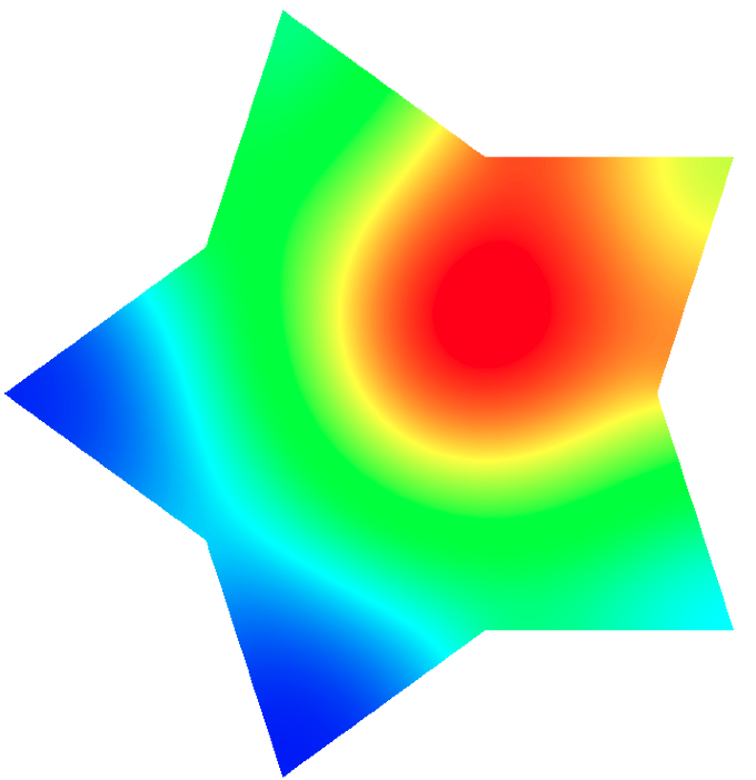
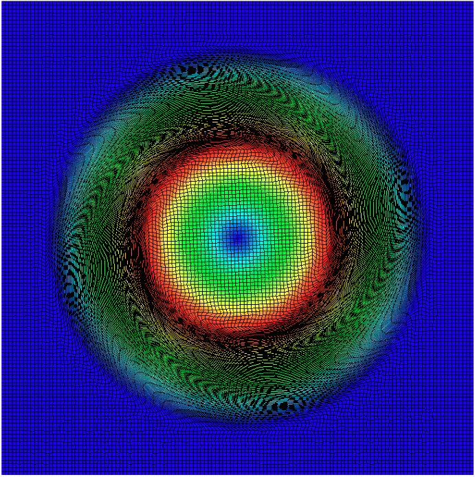
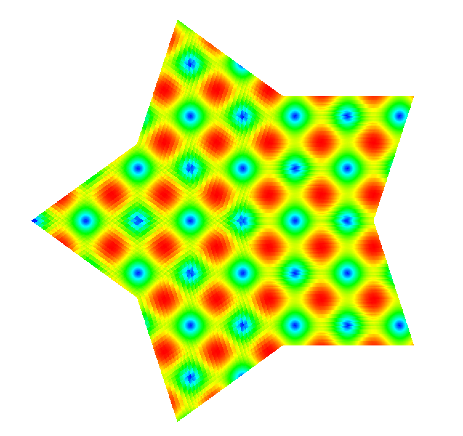
The 2D solution contour plot for $\kappa=\pi$ is shown in the figure
on the right to show the effect of $\kappa$. For demonstration, we sample
solutions at $\kappa=\pi$, $1.1\pi$, and $1.2\pi$. Then a ROM is build with basis size
of 3, which is used to predict the solution for $\kappa = 1.15\pi$. The ROM is
able to achieve a speedup of $7.5$ with a relative error of $6.4\times10^{-4}$.
One can follow the command line options below to reproduce the numerical results
summarized in the table below:
The command line option -f defines a frequency $\nu$ of the sinusoidal right hand
side function. The relation between $\kappa$ and the value $\nu$ specified by -f is defined as $\kappa = \pi
\nu$. The table below shows the performance result for the testing case -f 1.15.
FOM solution time
ROM solution time
Speed-up
Solution relative error
0.22 sec
0.029 sec
7.5
6.4e-4
The code that generates the numerical results above can be found in
(poisson_global_rom.cpp)
and the explanation of codes is provided in
here.
The
poisson_global_rom.cpp
is based on
ex1p.cpp from
MFEM with a modification on the right hand side function.
Greedy pROM for Poisson problem
This example code demonstrates physics-informed greedy sampling procedure of
building local pROMs for the Poisson problem. $$-\Delta u = f$$ with
homogeneous Dirichlet boundary conditions.
The example parameterizes
the righthand side with frequency variable, $\kappa$:
$$f =
\cases{
\displaystyle \sin(\kappa (x_0+x_1+x_2)) & for 3D \cr
\displaystyle \sin(\kappa (x_0+x_1)) & for 2D
}$$
A set of local ROMs are built for chosen parameter sample points. The parameter
sample points are chosen through physics-informed greedy procedure, which is
explained in detail by the tutorial YouTube
video. Then the local ROMs are interpolated to
build a tailored local ROM for a predictive case. Unlike the global ROM, the
interpolated ROM has dimension that is the same as the individual local ROM.
For example, one can follow the command line options below to reproduce the
numerical results summarized in the table below:
This particular greedy step generates local pROMs at the following 8 parameter points, i.e., 0.521923, 0.743108, 1.322449, 1.754950, 2.011140, 2.281129, 2.587821, 2.950198.
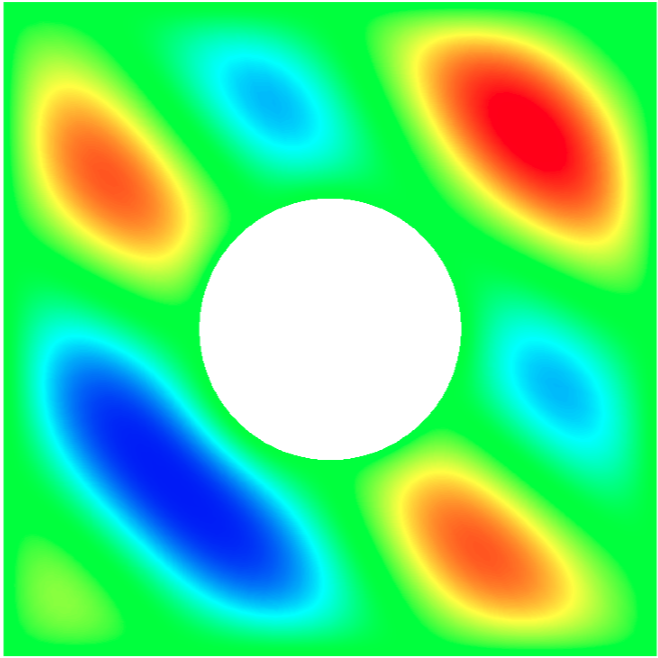
This example code demonstrates the use of libROM and MFEM to define a reduced
order model for a finite element discretization of the eigenvalue problem
$$-\text{div}(\kappa u) = \lambda u$$ with homogeneous Dirichlet boundary
conditions. The example parameterizes the diffusion operator on the left hand side
with the amplitude, $\alpha$:
The 2D solution contour plot for $\alpha=0.5$ is shown in the figure
on the right to show the effect of $\alpha$. For demonstration, we sample
solutions at $\alpha=0$ and $1$. Then a ROM is build with basis size
of 20, which is used to predict the solution for $\alpha = 0.5$. The ROM is
able to achieve a speedup of $375$ with a relative error of $6.7\times10^{-5}$ in the first
eigenvalue and $2.4 \times 10^{-3}$ in the first eigenvector.
One can follow the command line options below to reproduce the numerical results
summarized in the table below:
The command line option -a defines the amplitude of the conductivity $\alpha$
in the contrast region of the diffusion operator on left hand side.
The table below shows the performance result for the testing case -a 0.5.
with a natural insulating boundary condition $\frac{du}{dn}=0$. We linearize
the problem by using the temperature field $u$ from the previous time step to
compute the conductivity coefficient.
One can run the following command line options to reproduce the DMD results
summarized in the table below:
This example demonstrates the parametric DMD on the heat conduction
problem. The initial condition, $u_0(x)$, is
parameterized by the center of circle and the radius, i.e.,
$$u_0(x) =
\cases{
\displaystyle 2 & for $|x-c| < r$ \cr
\displaystyle 1 & for $|x-c| \ge r$
}$$
One can run the following command line options to reproduce the parametric DMD results
summarized in the table below:
Optimal control for heat conduction with DMD and differential evolution
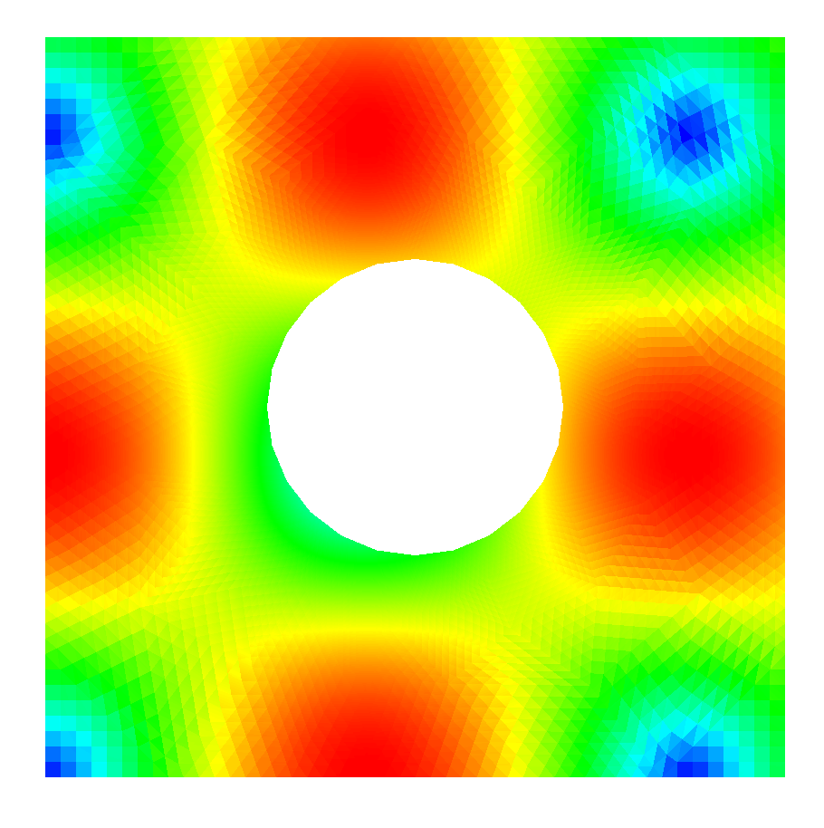
This example demonstrates the optimal control heat conduction problem with
greedy parametric DMD and differential evolution. The initial condition,
$u_0(x)$, is parameterized by the center of circle and the radius, i.e.,
$$u_0(x) =
\cases{
\displaystyle 2 & for $|x-c| < r$ \cr
\displaystyle 1 & for $|x-c| \ge r$
}$$
The goal of the optimal control problem is to find an initial condition that
achieves the target last time step temperature distribution. If it does not
achieve the target, then it should be closest, given the initial condition
parameterization. It is formulated mathematically as an optimization problem:
where $u_T$ denotes the last time step temperature and $u_{target}$ denotes the
target temperature. Note that $u_T$ depends on the initial condition
parameters, i.e., $c$ and $r$. It means that we obtain $u_T$ by solving a
forward heat conduction problem. As you can imagine, it needs to explore the
parameter space and try to find $c$ and $r$ that produces $u_T$ that best
matches $u_{target}$. If each solution process of heat conduction problem is
computationally expensive, the search for the optimal parameter can take a
while. Therefore, we use our parametric DMD to expedite the process and the
search algorithm is done by the differential
evolution.
Here are the steps to solve the optimal control problem. First, you must
delete any post-processed files from the previous differential evolution
run. For example,
rm -rf parameters.txt
rm -rf de_parametric_heat_conduction_greedy_*
Then create parametric DMD using a greedy approach with physics-informed error
indicator:
Then you can generate target temperature field with a specific $r$ and $c$
values. Here we used $r=0.2$, $cx=0.2$, and $cy=0.2$ to generate a target
temperature field. The target temperature field is shown in the picture above (the one on the left).
Therefore, if DMD is good enough, the differential evolution
should be able to find $c$ and $r$ values that are closed to these:
where r, cx, and cy specify the radius, the x and y coordinates of circular initial conditions.
Now you can run the differential evolution using the parametric DMD:
de_parametric_heat_conduction_greedy -r 0.2 -cx 0.2 -cy 0.2 -visit -de -de_f 0.9 -de_cr 0.9 -de_ps 50 -de_min_iter 10 -de_max_iter 100 -de_ct 0.001 (Run interpolative differential evolution to see if target FOM can be matched)
The differential evolution should be able to find the following optimal control parameters, e.g., in Quartz: $r=0.2002090156652667$, $cx=0.2000936529076073$, and $cy=0.2316380936755735$, which are close to the true parameters that were used to generate the targer temperature field. The DMD temperature field at the last time step on this control parameters is shown in the picture above (the one on the right).
with a natural insulating boundary condition $\frac{du}{dn}=0$ and an external inlet-outlet source
$$ f(x,t) = A_{+}(t) \exp\left(\dfrac{-| x - x_{+} |^2}{2}\right) - A_{-}(t) \exp\left(\dfrac{-| x - x_{-} |^2}{2}\right)), $$
where the source locations are $x_+ = (0, 0)$ and $x_- = (0.5, 0.5)$.
The amplitude $A_+$ and $A_-$ are regarded as control variables.
We linearize the problem by using the temperature field $u$ from the previous time step to
compute the conductivity coefficient.
One can run the following command line options to reproduce the DMDc results
summarized in the table below:
with a natural insulating boundary condition $\frac{\partial v}{\partial n}=0$. The
$H(div)$-conforming Raviart-Thomas finite element space is used for the velocity function $\boldsymbol{v}$,
and the $L^2$ finite element space is used for pressure function, $p$.
This example introduces how the hyper-reduction is implemented and how the
reduced bases for two field varibles, $p$ and $\boldsymbol{v}$.
One can run the following command line options to reproduce the pROM results
summarized in the table below:
where $c$ is advection velocity.
The initial condition, $u_0(x)$, is given by
$$u_0(x) =
\cases{
\displaystyle \exp\left (-\log(2)\frac{(x+7)^2}{0.0009}\right ) & for $-0.8 \le x \le -0.6$ \cr
\displaystyle 1 & for $-0.4 \le x \le -0.2$ \cr
\displaystyle 1-|10(x-0.1)| & for $0 \le x \le -0.2$ \cr
\displaystyle \sqrt{1-100(x-0.5)^2} & for $0.4 \le x \le 0.6$ \cr
\displaystyle 0 & \text{otherwise}
}$$
The DMD is applied to accelerate the advection simulation:
FOM solution time
DMD setup time
DMD query time
3.85 sec
0.18 sec
0.027 sec
The instruction of running this simulation can be found at
the HyPar page, e.g., go to Examples -> libROM Examples -> 1D Linear Advection-Discontinuous Waves.
DMD for wave equation
For a given initial condition, i.e., $u(0,x) = u_0(x)$,
and the initial rate, i.e. $\frac{\partial u}{\partial t}(0,x) = v_0(x)$,
wave equation solves the time-dependent hyperbolic problem:
$$\frac{\partial^2 u}{\partial t^2} - c^2 \Delta u = 0,$$
where $c$ is a given wave speed.
The boundary conditions are either Dirichlet or Neumann.
One can run the following command line options to reproduce the DMD results
summarized in the table below:
Optimal control for advection with DMD and differential evolution
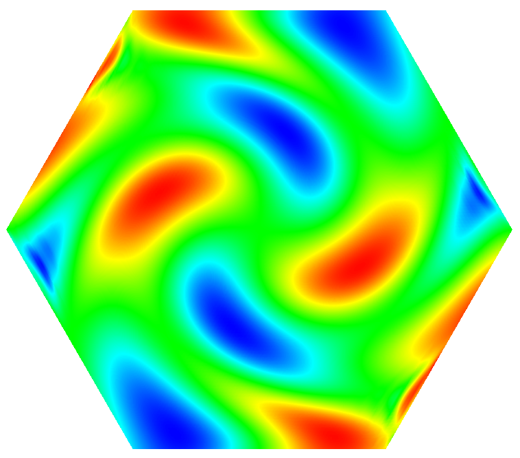
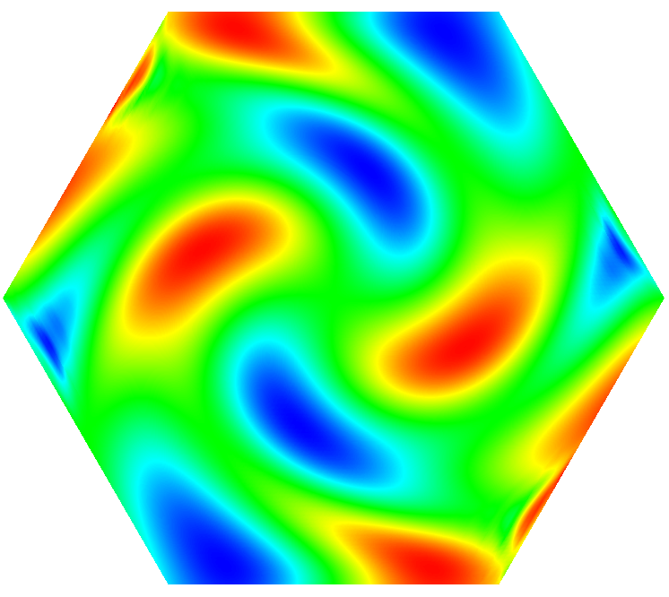
This example demonstrates optimal control for advection with the greedy
parametric DMD and differential evolution. The initial condition, $u_0(x)$,
is parameterized by the wavenumber $f$, so that
$$ u_0(x,y) = \sin(f \cdot x) sin(f \cdot y). $$
The goal of the optimal control problem is to find an initial condition that achieves the target
last time step solution. If it does not achieve the target, then it should be closest, given
the initial condition parameterization. It is formulated mathematically as an optimization problem:
where $u_T$ denotes the last time step solution and $u_{target}$ denotes the
target solution. Note that $u_T$ depends on the initial condition
parameter, $f$. It means that we obtain $u_T$ by solving a
forward advection problem. In order to do so, it must explore the
parameter space and try to find the $f$ that produces a $u_T$ that best
matches $u_{target}$. If each advection simulation is
computationally expensive, the search for the optimal parameter can take a
very long time. Therefore, we use our parametric DMD to expedite the process and the
search algorithm is done by differential
evolution.
Here are the steps to solve the optimal control problem. First, create a directory within which you
will run the example, such as
mkdir de_advection_greedy && cd de_advection_greedy
Then create the parametric DMD using a greedy approach with a physics-informed error indicator:
The differential evolution should be able to find the following optimal control parameters, e.g., in Quartz: $f = 1.597618121565086$, which is very close to the true parameter that was used to generate the targer solution. The images above show the the target solution on the left, and the DMD solution at the differential evolution optimal parameter on the right.
For a given initial condition, i.e., $u_0(x) = u(0,x)$,
DG advection solves the time-dependent advection problem:
$$\frac{\partial u}{\partial t} + v\cdot\nabla u = 0,$$
where $v$ is a given advection velocity.
We choose velocity function so that the dynamics form a spiral advection.
This example illustrates how a parametric pROM can be built through local ROM
interpolation techniques. The following sequence of command lines will let you
build such a parametric pROM, where the frequency of sinusoidal initial
condition function is used as a parameter (its value is passed by a user through -ff command line option).
Two local pROMs are constructed through -offline option with parameter values
of 1.02 and 1.08, then the local pROM operators are interpolated to build a
tailored local pROM at the frequency value of 1.05. Unlike the global ROM, the
interpolated pROM has dimension that is the same as the individual pROM, i.e.,
40 for this particular problem.
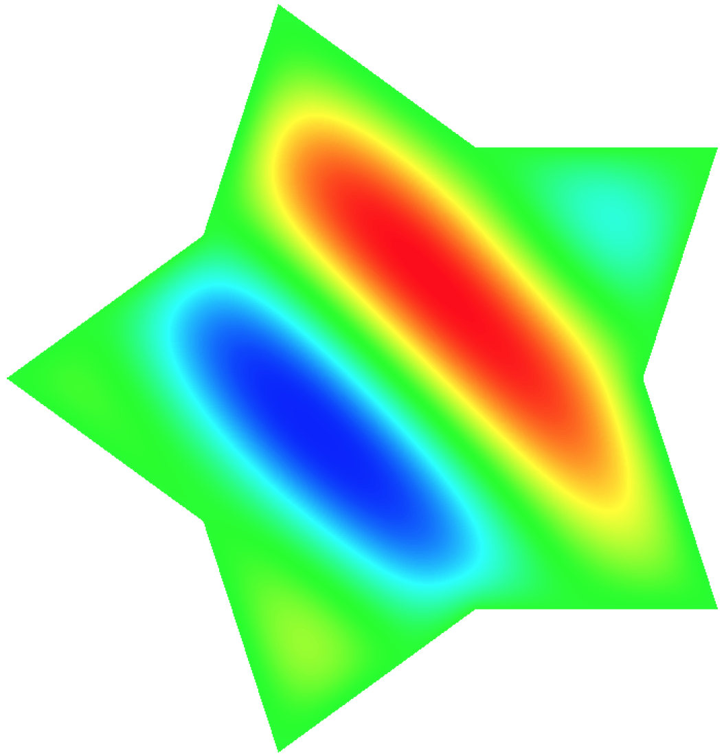
This example code demonstrates the use of libROM and MFEM to define a reduced
order model for a simple 2D/3D $H (\text{div})$ diffusion problem corresponding
to the second order definite equation
with boundary condition $F \cdot n = $ "given normal field."
The right-hand side $f$ is first calculated from the given exact solution $F$.
We then try to reconstruct the true solution $F$ assuming only the right-hand side function $f$ is known.
where $\kappa$ is a parameter controlling the frequency.
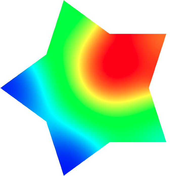
The 2D solution contour plot for $\kappa=1.15 \pi$ is shown in the figure
on the right to show the effect of $\kappa$. For demonstration, we sample
solutions at $\kappa=\pi$, $1.05\pi$, $1.1 \pi$, $1.2 \pi$, $1.25\pi$ and $1.3\pi$.
Then a ROM is built with basis size of 6, which is used to predict the solution
for $\kappa = 1.15\pi$. The ROM is able to achieve a speedup of $2.95\times10^5$ with a
relative error of $4.98\times10^{-8}$.
One can follow the command line options below to reproduce the numerical results
summarized in the table below:
The command line option -f defines the frequency of the sinusoidal right hand
side function. The relation between $\kappa$ and f is defined as $\kappa = \pi
f$.
$$ \rho = \left ( 1-\frac{(\gamma-1)b^2}{8\gamma \pi^2} e^{1-r^2} \right )^{\frac{1}{r-1}}, p = \rho^\gamma$$
$$ u = u_\infty - \frac{b}{2\pi} e^{\frac{1}{2}(1-r^2)}(y-y_c)$$
$$ v = v_\infty + \frac{b}{2\pi} e^{\frac{1}{2}(1-r^2)}(x-x_c),$$
where $b=0.5$ is the vortex strength and $r = \left ( (x-x_c)^2 + (y-y_c)^2 \right )^{\frac{1}{2}}$ is the distance from the vortex center $(x_c,y_c) = (5,5)$.
The DMD is applied to accelerate the vortex convection simulation:
FOM solution time
DMD setup time
DMD query time
5.85 sec
5.25 sec
0.28 sec
The instruction of running this simulation can be found at
the HyPar page, e.g., go to Examples -> libROM Examples -> 2D Euler Equations - Isentropic Vortex Convection.
is solved. The DMD is applied to accelerate the Riemann problem:
FOM solution time
DMD setup time
DMD query time
111.1 sec
17.6 sec
1.4 sec
The instruction of running this simulation can be found at
the HyPar page, e.g., go to Examples -> libROM Examples -> 2D Euler Equations - Riemann Problem Case 4
DMD for Euler equation
For a given initial condition, i.e., $u_0(x) = u(0,x)$,
DG Euler solves the compressible Euler system of equation, i.e., a model
nonlinear hyperbolic PDE:
with a state vector $\boldsymbol{u} = [\rho,\rho v_0, \rho v_1, \rho E]$, where
$\rho$ is the density, $v_i$ is the velocity in the $i$th direction, $E$ is the
total specific energy, and $H = E + p/\rho$ is the total specific enthalpy. The
pressure, $p$ is computed through a simple equation of state (EOS) call. The
conservative hydrodynamic flux $\boldsymbol{F}$ in each direction $i$ is
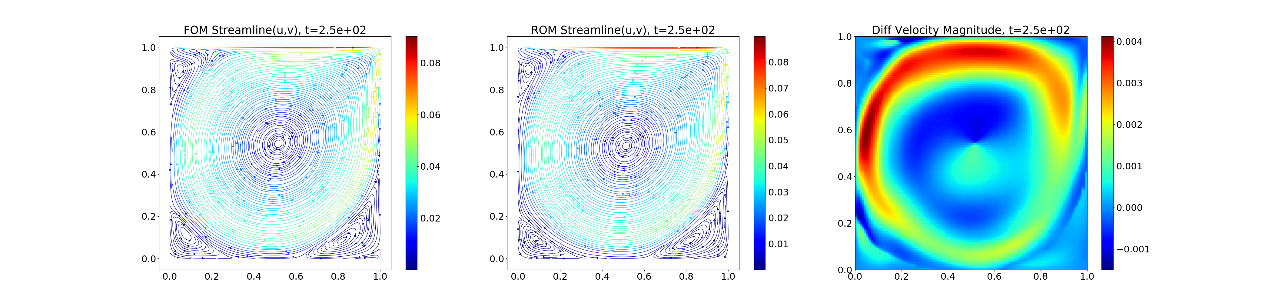
The DMD is applied to accelerate the cavity flow simulation:
FOM solution time
DMD setup time
DMD query time
554.6 sec
58.6 sec
0.3 sec
The instruction of running this simulation can be found at
the HyPar page, e.g., go to Examples -> libROM Examples -> 2D Navier-Stokes Equations - Lid-Driven Square Cavity
DMD for two-stream instability
The 1D-1V Vlasov equation is solved with the initial condition given by
The DMD is applied to accelerate the cavity flow simulation:
FOM solution time
DMD setup time
DMD query time
11.34 sec
2.30 sec
0.34 sec
The instruction of running this simulation can be found at
the HyPar page, e.g., go to Examples -> libROM Examples -> 2D (1D-1V) Vlasov Equation.
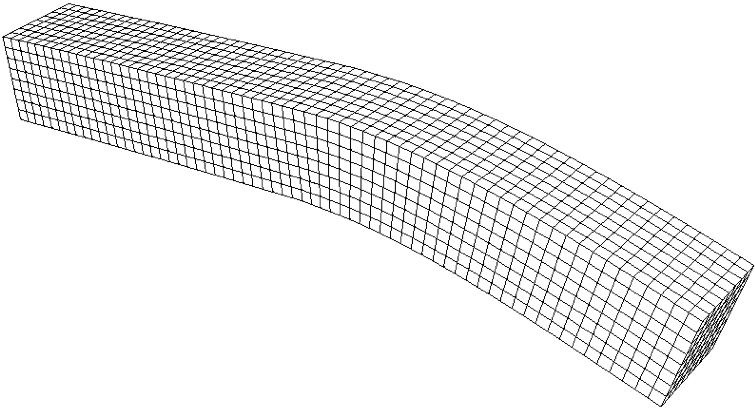
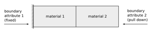
Global pROM for linear elasticity
This example demonstrates how to apply projection-based ROM to a linear
elasticity problem. The linear elasticity problem describes a multi-material
cantilever beam. Specifically, the following weak form is solved:
is the stress tensor corresponding to displacement field $\boldsymbol{u}$, and
$\lambda$ and $\mu$ are the material Lame constants. The Lame constants are
related to Young's modulus ($E$) and Poisson's ratio ($\nu$) as
The boundary condition are $\boldsymbol{u}=\boldsymbol{0}$ on the fixed part of the boundary with attribute 1, and $\sigma(\boldsymbol{u})\cdot n = f$ on the remainder with f being a constant pull down vector on boundary elements with attribute 2, and zero otherwise. The geometry of the domain is assumed to be as follows:
Three distinct steps are required, i.e., offline, merge, and online steps, to build global ROM for the linear elasticity problem. The general description of building a global ROM is explained in this YouTube tutorial video. We parameterized Poisson's ratio ($\nu$) from 0.2 to 0.4.
One can run the following command line options to reproduce the pROM results
summarized in the table below:
You can replace 0.XX with any value between 0.2 and 0.5. It must be strictly
less than 0.5. Note that the global ROM is able to predict the point outside of
the training region with high accuracy, i.e., $\nu=0.45$. The table below
shows the performance results for three different parameter points.
where $H$ is a hyperelastic model and $S$ is a viscosity operator of Laplacian
type. The initial displacement is set zero and the initial velocity is set as
zero except the third component which is defined:
$$v_3(0,x) = -\frac{\mu}{80}\sin(\mu x_1)$$
One can run the following command line options to build global ROM and
reproduce the results summarizedin the table below. You can replace XXX in the
fom and online phase to take any $\mu$ value between 3.9 and 4.1:
Laghos (LAGrangian High-Order Solver) is a miniapp that solves the
time-dependent Euler equations of compressible gas dynamics in a moving
Lagrangian frame using unstructured high-order finite element spatial
discretization and explicit high-order time-stepping. LaghosROM introduces
reduced order models of Laghos simulations.
A list of example problems that you can solve with LaghosROM includes Sedov
blast, Gresho vortex, Taylor-Green vortex, triple-point, and Rayleigh-Taylor
instability problems. Below are command line options for each problems and some
numerical results. For each problem, four different phases need to be taken,
i.e., the offline, hyper-reduction preprocessing, online, and restore phase. The
online phase runs necessary full order model (FOM) to generate simulation data.
libROM dynamically collects the data as the FOM simulation marches in time
domain. In the hyper-reduction preprocessing phase, the libROM builds a library
of reduced basis as well as hyper-reduction operators. The online phase runs the
ROM and the restore phase projects the ROM solutions to the full order model
dimension.
Sedov blast problem
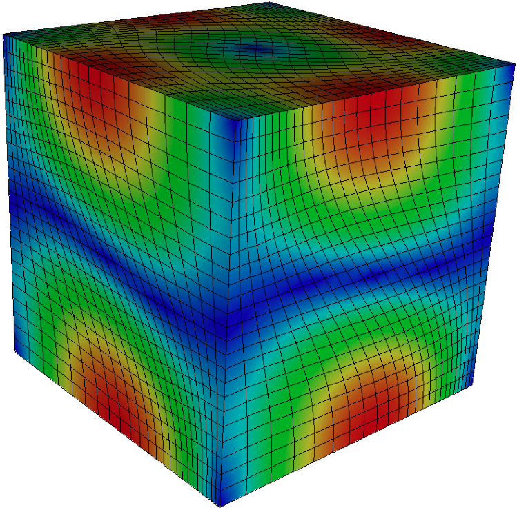
Sedov blast problem is a three-dimensional standard shock hydrodynamic
benchmark test. An initial delta source of internal energy deposited at the
origin of a three-dimensional cube is considered. The computational domain is
the unit cube $\tilde{\Omega} = [0,1]^3$ with wall boundary conditions on all
surfaces, i.e., $v\cdot n = 0$. The initial velocity is given by $v=0$. The
initial density is given by $\rho = 1$. The initial energy is given by a delta
function at the origin. The adiabatic index in the ideal gas equations of state
is set $\gamma = 1.4$. The initial mesh is a uniform Catesian hexahedral mesh,
which deforms over time. It can be seen that the radial symmetry is maintained
in the shock wave propagation in both FOM and pROM simulations. One can
reproduce the pROM numerical result, following the command line options
described below:
One can also easily apply time-windowing DMD to Sedov blast problem easily. First, prepare tw_sedov3.csv file, which contains a sequence of time steps, {0.01, 0.02, $\ldots$, 0.79, 0.8 } in a column. Then you can follow the command line options described below:
Gresho vortex problem is a two-dimensional benchmark test for the
incompressible inviscid Navier-Stokes equations. The computational domain is
the unit square $\tilde\Omega = [-0.5,0.5]^2$ with wall boundary conditions on
all surfaces, i.e., $v\dot n = 0$. Let $(r,\phi)$ denote the polar coordinates
of a particle $\tilde{x} \in \tilde{\Omega}$. The initial angular velocity is
given by
$$v_\phi =
\cases{
\displaystyle 5r & for 0 $\leq$ r < 0.2 \cr
\displaystyle 2-5r & for 0.2 $\leq$ r < 0.4 \cr
\displaystyle 0 i & for r $\geq$ 0.4.
}$$
The initial density if given by $\rho=1$. The initial thermodynamic pressure is
given by
$$p = \cases{
5 + \frac{25}{2} r^2 & for 0 $\leq$ r < 0.2 \cr
9 - 4 \log(0.2) + \frac{25}{2} - 20r + 4 \log(r) & for 0.2 $\leq$ r < 0.4 \cr
3 + 4\log(2) & for r $\geq$ 0.4 }$$
Taylor-Green vortex problem is a three-dimensional benchmark test for the
incompressible Navier-Stokes equasions. A manufactured smooth solution is
considered by extending the steady state Taylor-Green vortex solution to the
compressible Euler equations. The computational domain is the unit cube
$\tilde{\Omega}=[0,1]^3$ with wall boundary conditions on all surfaces,
i.e., $v\cdot n = 0$. The initial velocity is given by
The initial energy is related to the pressure and the density by the equation
of state for the ideal gas, $p=(\gamma-1)\rho e$, with $\gamma = 5/3$. The
initial mesh is a uniform Cartesian hexahedral mesh, which deforms over time.
The visualized solution is given on the right. One can reproduce the
numerical result, following the command line options described below:
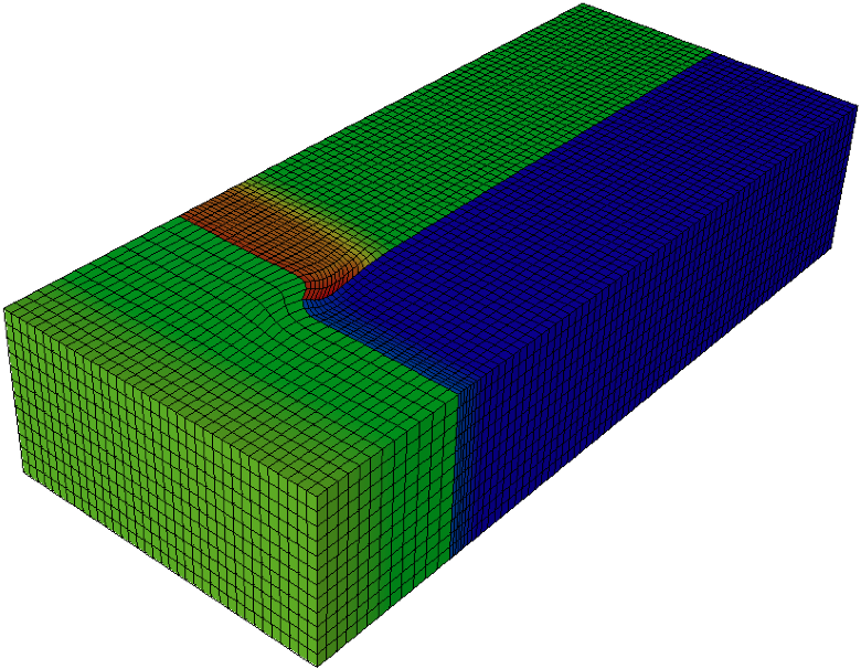
Triple-point problem is a three-dimensional shock test with two materials in
three states. The computational domain is $\tilde{\Omega} = [0,7] \times [0,3
] \times [0,1.5]$ with wall boundary conditions on all surfaces, i.e.,
$v\cdot n = 0$. The initial velocity is given by $v=0$. The initial density is
given by
$$\rho =
\cases{
\displaystyle 1 & for x $\leq$ 1 or y $\leq$ 1.5, \cr
\displaystyle 1/8 & for x $>$ 1 and y $>$ 1.5
}$$
The initial thermodynamic pressure is given for
$$p =
\cases{
\displaystyle 1 & for x $\leq$ 1, \cr
\displaystyle 0.1 & for x $>$ 1
}$$
The initial energy is related to the pressure and the density by the equation
of state for the ideal gas, $p=(\gamma-1)\rho e$, with
$$\gamma =
\cases{
\displaystyle 1.5 & for x $\leq$ 1 or y $>$ 1.5\cr
\displaystyle 1.4 & for x $>$ 1 and y $\leq$ 1.5
}$$
The initial mesh is a uniform Cartesian hexahedral mesh, which deforms over
time. The visualized solution is given on the right. One can reproduce the
numerical result, following the command line options described below:
This example builds a projection-based reduced-order model for an electromagnetic diffusion problem corresponding to the second order definite Maxwell equation
$$ \nabla \times \nabla \times \mathbf{E} + \mathbf{E} = \mathbf{f}.$$
The right-hand side function $\mathbf{f}$ is first calculated from a given exact vector field $\mathbf{E}$. We then try to reconstruct the true solution $\mathbf{E}$, assuming that we only know the right-hand side function $\mathbf{f}$.
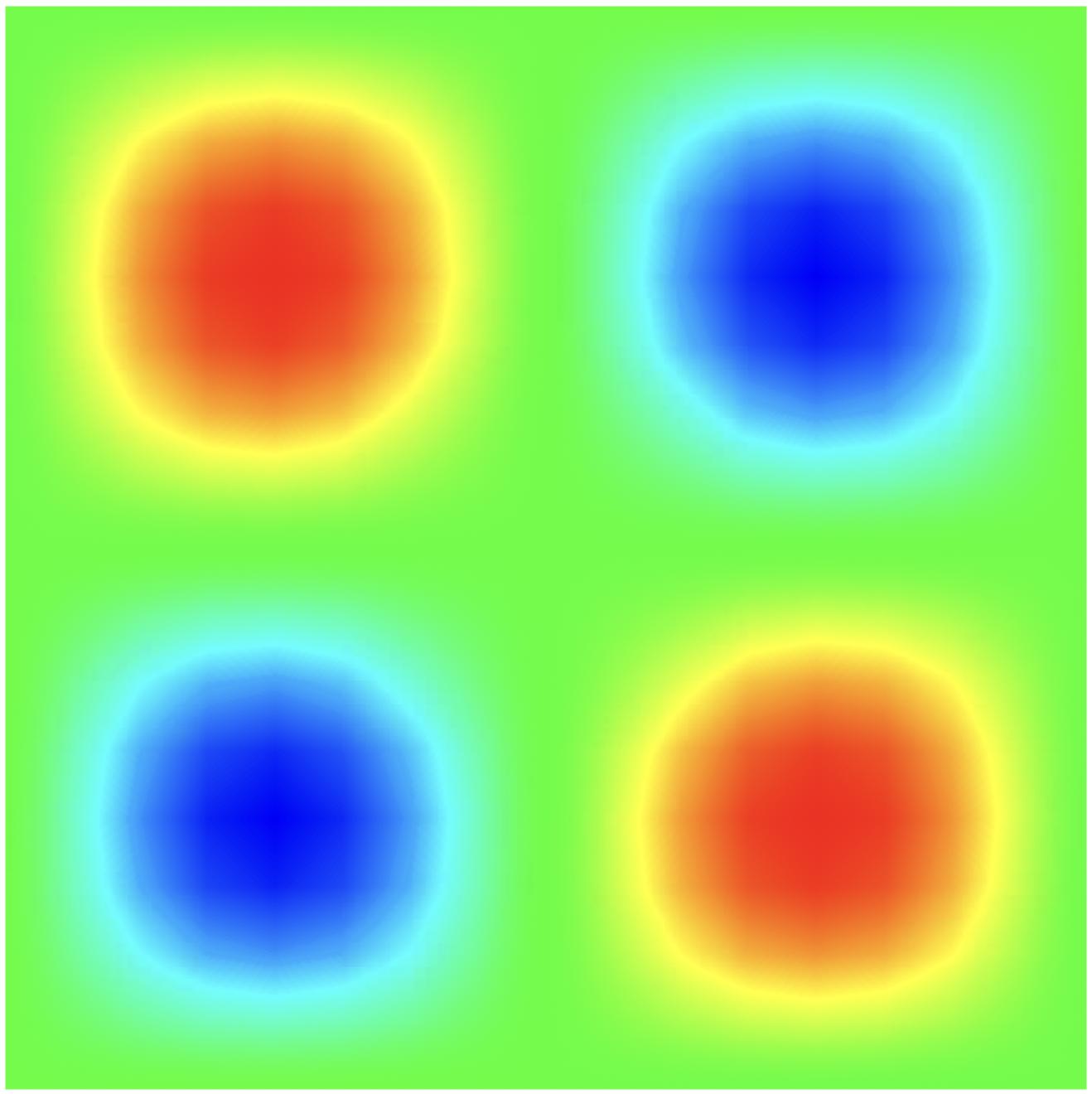
In 2D, we define $\mathbf{E}$ as
$$\mathbf{E} = (\sin ( \kappa x_2 ), \sin ( \kappa x_1 ) )^\top, $$
and in 3D we define
$$\mathbf{E} = (\sin ( \kappa x_2 ), \sin ( \kappa x_3 ), \sin ( \kappa x_1 ) )^\top. $$
Here, $\kappa$ is a parameter which controls the frequency of the sine wave.
The 2D solution contour plot for $\kappa= 1.15$ is shown in the figure on the right. For demonstration, we sample solutions at $\kappa=1\pi$, $1.1\pi$, and $1.2\pi$. We then build the ROM with a basis size of 3, which we use to predict the solution for $\kappa = 1.15$. The ROM is nearly $4856$ faster than the full-order model, with a relative error of $4.42\times10^{-4}$. One can follow the command line options to reproduce the numerical results summarized in the table below: