Poisson equation
The main code for this tutorial can be found in poisson_global_rom.cpp, which accelerates the Poisson problem $$-\Delta u = f$$ with homogeneous Dirichlet boundary conditions. The numerical results can be found in Poisson Problem.
libROM assumes that you have a physics code, such as MFEM, SU2, and Laghos. Then, libROM can be integrated into the physics code to build ROM to accelerate physics simulation. For example, see numerical results in Examples and Gallery. This tutorial illustrates how various libROM objects and functions can be used to collect simulation data, build reduced basis, and construct reduced order model operator to accelerate and predict a target physics simulation.
The following tutorials are available:
- Tutorial 1: offline, Take and write simulation data with libROM.
- Tutorial 2: merge, Collect simulation data and build a reduced basis.
- Tutorial 3: online, Build a ROM operator, solve the ROM system, and restore the full order state.
Building
Follow the building page to build the libROM library. You must build it with -m option to build MFEM library together.
~/libROM> ./scripts/compile.sh -m
Tutorial 1
This tutorial demonstrates how to collect simulation data with libROM. The important object is BasisGenerator, which collects simulation data and computes reduced basis, using various singular value decomposition (SVD) algorithms, e.g., incremental SVD and static SVD. The incremental SVD is useful for time-dependent problems. Because the Poisson problem is a time-independent problem, we will focus on the usage of the static SVD. The definition of BasisGenerator class can be found in BasisGenerator.h.
You must include BasisGenerator.h in your physics code where the simulation data is generated. For example, BasisGenerator.h is included in Line 32 of poisson_global_rom.cpp for Poisson Problem.
#include "BasisGenerator.h"
A BasisGenerator pointer is defined in Line 234 of poisson_global_rom.cpp and the pointer is initiated in Line 243 of poisson_global_rom.cpp. The BasisGenerator requires four inputs to initialize, i.e., Options, boolean variable, string, and Database::formats. The object, Options, sets various options for the BasisGenerator, such as the basis dimension and singular value tolerance. The boolean variable determines if the incremental or static SVD will be used. For this tutorial, we choose the static SVD, so the boolean variable must be false. Finally, the string input specifies the name of the basis file and Database::formats specifies the file format for the basis file. The default format is Database::HDF5. The detailed description for inputs for Options and BasisGenerator can be found in Options.h and BasisGenerator.h. The specific inputs used for the Poisson problem can be found in Lines 227--232 of poisson_global_rom.cpp.
Now, the instantiated BasisGenerator, i.e., generator, collects the simulation data once it is available. The Poisson problem generates the solution, $X$, in Line 338 of poisson_global_rom.cpp and it is collected in the generator in Line 345 of poisson_global_rom.cpp. The member function, writeSnapshot on Line 346 of poisson_global_rom.cpp simply writes the solution data in the specified HDF5 file. Make sure that the pointers, generator and options, are deleted after done with sampling. This completes the libROM data collection implementation, which corresponds to the offline phase in the Poisson problem. If you execute the following command:
poisson_global_rom -offline -f 1.0 -id 0
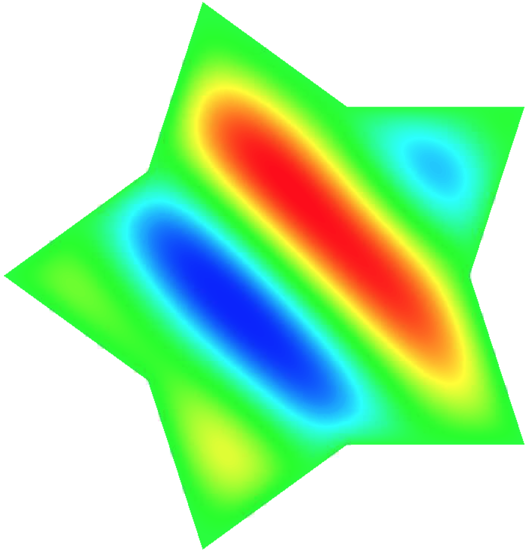
then you should see the HDF5 snapshot output file, i.e., basis0_snapshot.000000. The command line options above include -offline that indicates the offline phase, -f 1.0 sets the frequency variable $\kappa=1.0$ (see the Poisson problem for the description of the frequency variable), and -id 0 labels the snapshot index. The visualization of the solution can be done either with VisIt or GLVis. For example, the VisIt shows the following solution contour for this specific simulation:

Please execute the following commands:
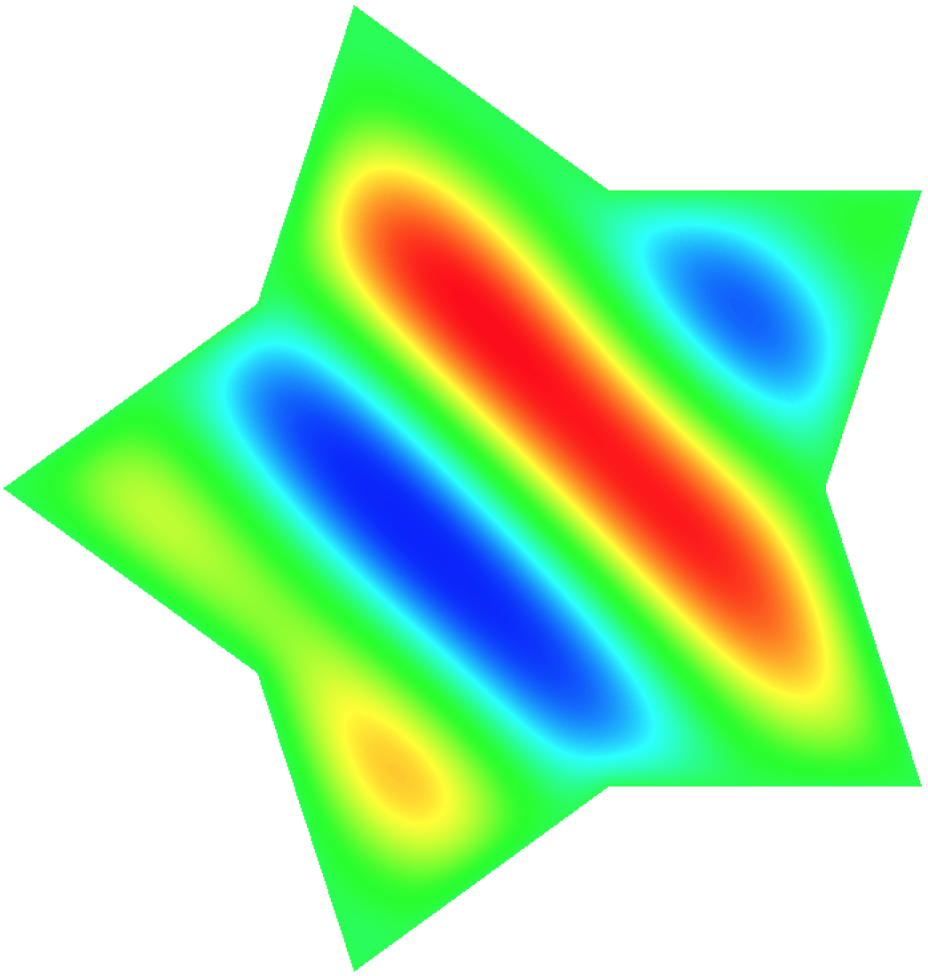
poisson_global_rom -offline -f 1.1 -id 1
poisson_global_rom -offline -f 1.2 -id 2
whose solution contour corresponds, respectively, to:
Tutorial 2
Once the simulation data are collected within libROM basis files, they can be merged to form a reduced basis. This process is called the merge phase. It is implemented in Lines 249--270 of poisson_global_rom.cpp. As in Tutorial 1, the objects, Options and BasisGenerator must be defined (see Lines 251--253 of poisson_global_rom.cpp. The generator iterates over the individual HDF5 snapshot file and loads them all (see Lines 254--259 of poisson_global_rom.cpp. The member function endSamples in Line 260 of poisson_global_rom.cpp computes the reduced basis. Again make sure to delete the pointers, i.e., generator and options.
For exammple, the following command line option runs the merge phase:
poisson_global_rom -merge -ns 3
The command line option, -merge, invokes the merges phase and -ns 3 option indicates that there are three different snapshot files. The merge phase reads the three snapshot files, i.e., basis0_snapshot.000000, basis1_snapshot.000000, and basis2_snapshot.000000, which were generated in Tutorial 1, and forms a reduced basis and stores it in the HDF5 basis file, i.e., basis.000000.
Tutorial 3
The online phase builds ROM operators, solves the ROM system, and restores the full order states for a new parameter value. This tutorial demonstrates these three different actions for the frequency value, $\kappa = 1.15$.
Lines 356--357 of poisson_global_rom.cpp implements the step of reading a basis file. The BasisReader object reads the basis file, using member function, getSpatialBasis, which returns a Matrix object in libROM. The number of rows and columns of the reduced basis can be obtained through the member functions of the Matrix class, i.e., numRows and numColumns, respectively.
Line 364 of poisson_global_rom.cpp defines a MFEM DenseMatrix that holds the transpose of the reduced basis matrix. This must be understood as the transpose because libROM stores the matrix row-wise. The MFEM matrix is defined to form a reduced system operator, whose process is implemented in Lines 368--375 of poisson_global_rom.cpp. Then the reduced system operator is inverted at Line 370 of poisson_global_rom.cpp.
The reduced right-hand-side is formed by multiplying the reduced basis transpose to the full order model right-hand-side vector, $B$ at Line 374 of poisson_global_rom.cpp.
Line 380 of poisson_global_rom.cpp solves the reduced system of equation.
Line 384 of poisson_global_rom.cpp restores the corresponding full order state by multipling the reduced solution by the reduced basis.
The command line options that executes the online phase described above are
poisson_global_rom -online -f 1.15
where -online option invokes the online phase and -f 1.15 sets the frequency value $\kappa = 1.15$. This particular example ROM accelerates the physics simulation by $7.5$ and achieves the relative error, $6.4e-4$, with respect to the corresponding full order model solution.