Features
The goal of libROM is to provide high-performance scalable library for data-driven reduced order modeling.
Proper orthogonal decomposition
One of the core features in libROM is the ability to extract important modes from given physical simulation data. The proper othogonal decomposition (POD) is a popular method for compressing physical simulation data to obtain optimal "reduced" bases in the following sense:
$$\boldsymbol{\Phi} =\underset{\boldsymbol{A}\in\mathbb{R}^{n\times r}, \boldsymbol{A}^T\boldsymbol{A} = \boldsymbol{I}_{r\times r} }{\arg\min} || \boldsymbol{U} - \boldsymbol{A}\boldsymbol{A}^T\boldsymbol{U} ||_F^2, $$
where $\boldsymbol{U}\in\mathbb{R}^{n\times m}$ is simulation data and $\boldsymbol{I}_{r\times r} \in \mathbb{R}^{r\times r}$ denotes an identity matrix. That is, the POD tries to find the orthogonal matrix, $\boldsymbol{\Phi}$, whose span minimizes the projection error in the Frobenius norm. The POD modes can be obtained in two equivalent ways: (i) eigenvalue decomposition and (ii) singular value decomposition (SVD). We take the latter approach, i.e., let's say the thin SVD of $\boldsymbol{U}$ is given by
$$\boldsymbol{U} = \boldsymbol{W\Sigma V}^T.$$
Then the solution of the POD is given by taking the first $r$ columns of the left singular matrix, i.e., $\boldsymbol{\Phi} = [\boldsymbol{w}_{1},\ldots ,\boldsymbol{w}_r]$, where $\boldsymbol{w}_k$ is $k$th left singular vector, assuming that the singular value is written in the decreasing order.
Efficient data collection
High-fidelity physical simulations generate intensive data in its size, which makes the data collection process daunting. Therefore, the libROM aims to ease the difficulty associated with the intensive data size.
The libROM can be directly integrated to the physics solver that generates the intensive simulation data. For example, if the physical simulation is time dependent, then each time step solution data can be feed into the libROM incrementally so that the singular value decomposition is efficiently updated in parallel. This approach is incremental SVD. There are other types of SVDs which exploits efficiency. The libROM provides following four SVDs:
- Static SVD
- incremental SVD
- randomized SVD
- space-time SVD
Static SVD
The static SVD waits the libROM to collect all the simulation data. Once the snapshot matrix $\boldsymbol{U}$ is formed, then the SVD is performed. Therefore, if the data size is big, this approach is not efficient and not recommended. However, because it gives the most accurate SVD results, it is ideal for a small problem.
Incremental SVD
Unlike the static SVD, the incremental SVD does not wait. Instead, as the data comes in, the SVD is performed right away. Because the incremental SVD only needs to find out the effect of one additional simulation data vector to the previous SVD, the update can be done very efficiently without requiring much memory. Therefore, it is useful for large-scale problems. For the detailed explanation about the incremental SVD, we refer to the following journal papers:
- M. Brand, Incremental singular value decomposition of uncertain data with missing values, In European Conference on Computer Vision, p707-720, 2002
- G. Oxberry, T. Kostova-Vassilevska, W. Arrighi, K. Chand, Limited-memory adaptive snapshot selection for proper orthogonal decomposition, International Journal for Numerical Methods in Engineering, 109(2), p198-217, 2016
- H. Fareed, J.R. Singler, Error Analysis of an Incremental Proper Orthogonal Decomposition Algorithm for PDE Simulation Data, Journal of Computational and Applied Mathematics, 368, 112525, 2020
Randomized SVD
Randomization can bring computational efficiency in computing SVDs. For example, consider that one needs to extract $p$ dominant modes from $n \times m$ tall dense matrix, using SVD. The randomized SVD requires $\mathcal{O}(nm\log(p))$ floating-point operations, while the static SVD algorithm requires $\mathcal{O}(nmp)$ flops. The randomized SVD that is implemented in libROM can be found in the following journal paper:
- N. Halko, P.G. Martinsson, J.A. Tropp, Finding structure with randomness: Probabilistic algorithms for constructing approximate matrix decompositions. SIAM review, 53(2), p217-288, 2011
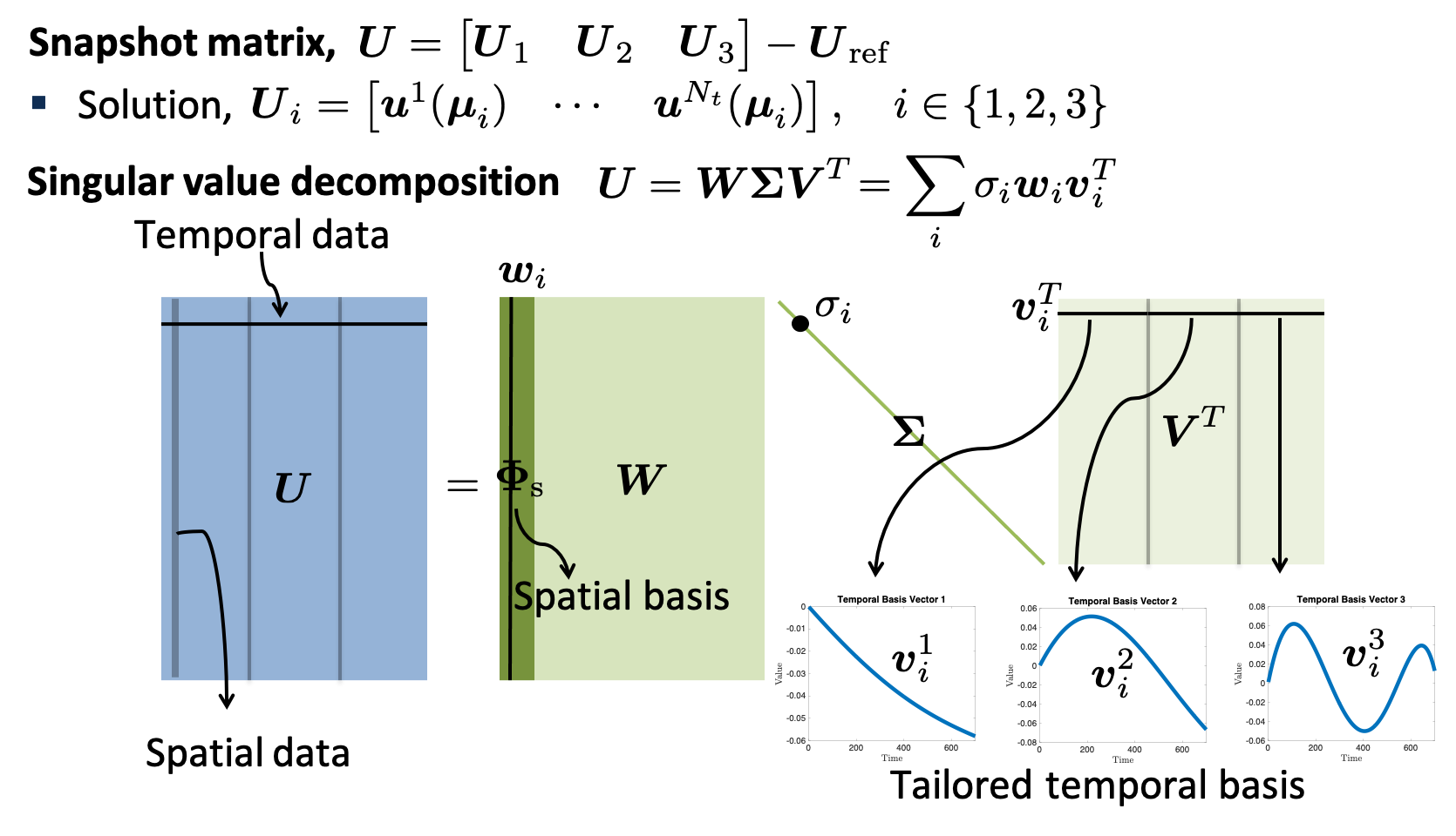
Space-time SVD
For time dependent problems, one can reduce not only the spatial degrees of freedom, but also the temporal degrees of freedom by representing the space-time solution as a linear combination of a space-time reduced basis. The space-time reduced basis can be mathematically written as a Kronecker product of temporal and spatial bases. Fortunately, one can extract temporal as well as spatial reduced bases from one single SVD. The procedure is schematically depicted in the figure below:
For the detailed explanation about the incremental SVD, we refer to the following three journal papers:
- Y. Kim, K. Wang, Y. Choi, Efficient space–time reduced order model for linear dynamical systems in Python using less than 120 lines of code. Mathematics, 9(14), 1690, 2021
- Y. Choi, P. Brown, W. Arrighi, R. Anderson, K. Huynh, Space–time reduced order model for large-scale linear dynamical systems with application to boltzmann transport problems. Journal of Computational Physics, 424, 109845, 2021
- Y. Choi, K. Carlberg, Space-time least-squares Petrov-Galerkin projection for nonlinear model reduction, SIAM Journal on Scientific Computing, 41(1), A26-A58, 2019
Dynamic Mode Decomposition
The dynamic mode decomposition (DMD) provides a great way of finding an approximate locally linear dynamical system,
$$ \frac{d\boldsymbol{u}}{dt} = \mathcal{A}\boldsymbol{u},$$
for a given nonlinear dynamical system,
$$ \frac{d\boldsymbol{u}}{dt} = \boldsymbol{f}(\boldsymbol{u},t;\boldsymbol{\mu}),$$
with initial condition, $\boldsymbol{u}_0$. It takes non-intrusive approach, i.e., equation-free method, so it is applicable even if there is only data, but no $\boldsymbol{f}(\boldsymbol{u},t;\boldsymbol{\mu})$. For example, let's say the discrete-time data are given as:
$$\boldsymbol{U} = [\boldsymbol{u}_1,\ldots,\boldsymbol{u}_m],$$
where $\boldsymbol{u}_k\in\mathbb{R}^n$ denotes solution at $t=k\Delta t$. The DMD is trying to find the best $\boldsymbol{A}$ such that
$$\boldsymbol{U}^+ = \boldsymbol{A}\boldsymbol{U}^-,$$
where $\boldsymbol{U}^+ = [\boldsymbol{u}_2,\ldots,\boldsymbol{u}_m]$ and $\boldsymbol{U}^- = [\boldsymbol{u}_1, \ldots, \boldsymbol{u}_{m-1}]$. The following procedure is taken to find the best $\boldsymbol{A}$.
-
Take the singular value decomposition (SVD) of $\boldsymbol{U}^-$
$$\boldsymbol{U}^- \approx \boldsymbol{W}\boldsymbol{\Omega}\boldsymbol{V}^*,$$
where $*$ denotes the conjugate transpose, $\boldsymbol{W}\in\mathbb{C}^{n\times r}$, $\boldsymbol{\Omega}\in\mathbb{C}^{r\times r}$, $\boldsymbol{V}\in\mathbb{C}^{m\times r}$, and $r \leq m$.
-
Because $\boldsymbol{U}^+ = \boldsymbol{A}\boldsymbol{U}^-$, using the pseudo-inverse of the approximate $\boldsymbol{U}^-$, we have
$$\boldsymbol{A} \approx \tilde{\boldsymbol{A}} = \boldsymbol{U}^+\boldsymbol{V}\boldsymbol{\Omega}^{-1}\boldsymbol{W}^*$$
-
It is easier to deal with the reduced operator $\tilde{\boldsymbol{A}}_r$, which relates the discrete-time dynamic of reduced states:
$$\tilde{\boldsymbol{u}}_{k+1} = \tilde{\boldsymbol{A}}_r\tilde{\boldsymbol{u}}_k,$$
where $\boldsymbol{u}_k = \boldsymbol{W} \tilde{\boldsymbol{u}}_k$ and $\tilde{\boldsymbol{A}}_r$ is defined as
$$\tilde{\boldsymbol{A}}_r=\boldsymbol{W}^*\tilde{\boldsymbol{A}}\boldsymbol{W}$$
$$\tilde{\boldsymbol{A}}_r=\boldsymbol{W}^*\boldsymbol{U}^+\boldsymbol{V}\boldsymbol{\Omega}^{-1}$$
-
Let the eigen-decomposition of $\tilde{\boldsymbol{A}}_r$ to be
$$\tilde{\boldsymbol{A}}_r \boldsymbol{X} = \boldsymbol{X}\boldsymbol{\Lambda}$$
and set either $\boldsymbol{\Phi} = \boldsymbol{W}\boldsymbol{X}$ or $\boldsymbol{\Phi} = \boldsymbol{U}^+ \boldsymbol{V} \boldsymbol{\Omega}^{-1}\boldsymbol{X}$, then the DMD solution at time, $t$, can be found as
$$\boldsymbol{u}(t) = \boldsymbol{\Phi}\boldsymbol{\Lambda}^{t/\Delta t} \boldsymbol{b}_0,$$
where $\boldsymbol{b}_0 = \boldsymbol{\Phi}^\dagger \boldsymbol{u}_0$.
For the detailed explanation about the DMD, we refer to the following book:
- J.N. Kutz, S.L. Brunton, B.W. Brunton, J.L. Proctor, Dynamic mode decomposition: data-driven modeling of complex systems. Society for Industrial and Applied Mathematics, 2016
Projection-based reduced order model
In contrast to the DMD, the projection-based reduced order model (pROM) takes an intrusive approach, that is, it is NOT equation-free. The pROM first represents the solution as a linear combincation of reduced basis. The reduced basis can be obtained by the POD, for example. Let's denote the reduced basis as $\boldsymbol{\Phi}\in\mathbb{R}^{n\times r}$ and express the solution, $\boldsymbol{u}\in\mathbb{R}^n$ as
$$\boldsymbol{u} = \boldsymbol{u}_{\text{ref}}+\boldsymbol{\Phi}\hat{\boldsymbol{u}},$$
where $\hat{\boldsymbol{u}} \in \mathbb{R}^r$ denotes the generalized coordinates with respect to the reduced basis. Then we substitute $\boldsymbol{u}$ in the governing equation, say a nonlinear dynamical system governed by the following ordinary differential equations,
$$\frac{d\boldsymbol{u}}{dt} = \boldsymbol{f}(\boldsymbol{u},t;\boldsymbol{\mu}),$$
to obtain the over-determined system, i.e.,
$$\boldsymbol{\Phi}\frac{d\hat{\boldsymbol{u}}}{dt} = \boldsymbol{f}(\boldsymbol{u}_{\text{ref}}+\boldsymbol{\Phi}\hat{\boldsymbol{u}},t;\boldsymbol{\mu}),$$
which has more equations than unknowns. Therefore, the system needs to be closed by a projection. Galerkin and Petrov-Galerking projections are popular. For example, the Galerkin projection multiplies both sides by $\boldsymbol{\Phi}^T$ and the system of equations become
$$\frac{d\hat{\boldsymbol{u}}}{dt} = \boldsymbol{\Phi}^T \boldsymbol{f}(\boldsymbol{u}_{\text{ref}}+\boldsymbol{\Phi}\hat{\boldsymbol{u}},t;\boldsymbol{\mu})$$
By the way, the nonlinear term $\boldsymbol{f}$ still scales with the full order model size and it needs to be updated every time its argument changes due to Newton step updates, for example. The hyper-reduction provides an efficient way of computing nonlinear terms by sampling an important subset. By the way, if $\boldsymbol{f}$ is linear, then $\boldsymbol{\Phi}^T\boldsymbol{f}$ can be pre-computed, so the hyper-reduction is not necessary.
Hyper-reduction
Hyper-reduction is essential to reduce the complexity of nonlinear terms in pROM. The most popular hyper-reduction technique is the discrete empirical interpolation method (DEIM). The DEIM approximates the nonlinear term with a gappy POD, i.e., it expresses the nonlinear term with a linear combination of the nonlinear term reduced basis, $\boldsymbol{\Phi}_{f}\in\mathbb{R}^{n\times f}$:
$$\boldsymbol{f} \approx \boldsymbol{\Phi}_f \hat{\boldsymbol{f}},$$
where $\hat{\boldsymbol{f}}\in\mathbb{R}^{f}$ is a generalized coordinate for the nonlinear term. The usual data for the nonlinear term basis, $\boldsymbol{\Phi}_{f}$ is snapshot of nonlinear term itself. Alternatively, it can be replaced by the solution basis (i.e., $\boldsymbol{\Phi}$ or slight modification of it) via the SNS method introduced in the following journal paper:
- Y. Choi, D. Coombs, R. Anderson, SNS: a solution-based nonlinear subspace method for time-dependent model order reduction. SIAM Journal on Scientific Computing, 42(2), A1116–A1146, 2020
Then, we introduce a sampling matrix (in order words, a collocation matrix), $\boldsymbol{Z}\in\mathbb{R}^{n\times z}$, which selects a subset of the nonliear term, $\boldsymbol{F}$. That is, each column of $\boldsymbol{Z}$ is a column of the identity matrix, $\boldsymbol{I} \in \mathbb{R}^{n\times n}$. Combining the collocation matrix and the nonlinear basis, we solve the following least-squares problem to solve for the generalized coordinate, $\hat{\boldsymbol{f}}$:
$$\hat{\boldsymbol{f}} = \underset{\boldsymbol{y}\in{\mathbb{R}^{f}}}{\arg\min} \hspace{3pt} || \boldsymbol{Z}^T\boldsymbol{f} - \boldsymbol{Z}^T\boldsymbol{\Phi}_f \boldsymbol{y} ||_2^2$$
The solution to the least-squares problem is known to be
$$\hat{\boldsymbol{f}} = (\boldsymbol{Z}^T\boldsymbol{\Phi}_{f})^\dagger \boldsymbol{Z}^T\boldsymbol{f}.$$
Note that $(\boldsymbol{Z}^T\boldsymbol{\Phi}_{f})^\dagger$ can be pre-computed once the indices for $\boldsymbol{Z}$ and $\boldsymbol{\Phi}_f$ are known. Note also that you do not need to construct $\boldsymbol{Z}$. You only need to sample selected rows of $\boldsymbol{\Phi}_f$ and do the pseudo-inversion. This is what we do in libROM. Also note that we only need to evaluate a subset of $\boldsymbol{f}$ because of $\boldsymbol{Z}^T$ in front of $\boldsymbol{f}$.
Parametric ROMs
Whether it is intrusive or non-intrusive ROM, if the ROM can only reproduce the full order model simulation data with high accuracy, it is useless because the full order model solution is already available. In order for any ROMs to be useful, they must be able to predict the solution which is not generated yet. We call such a ROM parametric because it is able to predict the solution for a new parameter value. Two extreme types of parametric ROMs are global and local ROMs.
Global ROMs
The global ROMs collect simulation data over several sampled points in a given parameter space and use all of them as a whole, building a global reduced basis. The size of the reduced basis becomes larger as the number of samples increases. Therefore, the global ROM is only effective when a small number of samples are used.
Local ROMs
A local ROM is built with the simulation data corresponding only to one specific sample. Usually, several local ROMs are built for several sample points and either interpolation or trust-region is used to predict the solution at points which were not sampled.
Greedy sampling algorithm
The greedy sampling algorithm is a physics-informed sampling strategy to build a parametric ROM. The parametric ROM can be used to predict the solution of a new parameter point that has not been seen in the training phase. The greey algorithms follow the general procedure below:
- Define a parameter space
- Pick an initial point in the parameter space to build a ROM there (a good cancidiate initla point is either the centroid or one of end points)
- Evaluate error indicator of the current ROM (either global or local ROM) at $N$ random points within the parameter space
- Check if the maximum error indicator value is less than the desirable accuracy threshold
- If the answer to Step 4 is yes, then terminate the greedy process.
- If the answer to Step 4 is no, then collect the full order model simulation data at the maximum error indicator point and add them to update the ROM
- Go to Step 3.
The success of the greedy algorithm depends on the error indicator. The error indicator must satisfy the following two criteria:
- Its value must have positive correlation with the relative error measure
- The evaluation of the error indicator must be computationally efficient
Note that the error indicator plays a role of a proxy for the accuracy of the ROM. The most popular error indicator is residual-based, which we recommend you to use for your physical simulations.
The general framework of the greedy algorithm is implemented in libROM. The example of the libROM usage case can be found for the Poisson problem at poisson_greedy.cpp. The corresponding tutorial page can be found here.
Several variants of the greedy procedure described above is possible. For more detailed explanation about the greedy algorithm, we refer to the following jounral paper, where the greedy algorithm is described for the interpolated ROM in a matrix manifold:
- Y. Choi, G. Boncoraglio, S. Anderson, D. Amsallem, C. Farhat, Gradient-based constrained optimization using a database of linear reduced order models. Journal of Computational Physics, 423, 109787, 2020
We recommend another excellent paper for the greedy algorithm:
- A. Paul-Dubois-Taine, D. Amsallem, An adaptive and efficient greedy procedure for the optimal training of parametric reduced-order models. International Journal for Numerical Methods in Engineering, 102, p1262-1292, 2014
Latent Space Dynamics Identification
Latent Space Dynamics Identification (LaSDI) is a reduced order model framework that follows three distinct steps: compression, identification, and prediction. For compression, LaSDI employs both linear and nonlinear techniques. For identification, it uses sparse regression methods, such as SINDy and weak-form SINDy, or adopts a fixed form, like the neural network version of GENERIC formalism (i.e., GFINN).
We recommend the followin excellent papers for LaSDI framework:
- W.D. Fries, X. He, and Y. Choi, Lasdi: Parametric latent space dynamics identification. Computer Methods in Applied Mechanics and Engineering, 399, p.115436, 2022
- X. He, Y. Choi, W.D. Fries, J.L. Belof, J.S. Chen, gLaSDI: Parametric physics-informed greedy latent space dynamics identification. Journal of Computational Physics, 489, p.112267. 2023
- C. Bonneville, Y. Choi, D. Ghosh, J.L. Belof, GPLaSDI: Gaussian process-based interpretable latent space dynamics identification through deep autoencoder. Computer Methods in Applied Mechanics and Engineering, 418, p.116535, 2024
- A. Tran, X. He, D.A. Messenger, Y. Choi, D.M. Bortz, Weak-form latent space dynamics identification. Computer Methods in Applied Mechanics and Engineering, 427, p.116998, 2024
- J.S.R. Park, S.W. Cheung, Y. Choi, Y. Shin, tLaSDI: Thermodynamics-informed latent space dynamics identification. arXiv preprint arXiv:2403.05848, 2024
- C. Bonneville, X. He, A. Tran, J.S. Park, W. Fries, D.A. Messenger, S.W. Cheung, Y. Shin, D.M. Bortz, D. Ghosh, J.S. Chen, A Comprehensive Review of Latent Space Dynamics Identification Algorithms for Intrusive and Non-Intrusive Reduced-Order-Modeling. arXiv preprint arXiv:2403.10748, 2024
Domain Decomposition Nonlinear Manifold Reduced Order Model
Domain Decomposition Nonlinear Manifold Reduced Order Model (DD-NM-ROM) constructs local nonlinear manifold reduced order models in space to mitigate the high computational cost of neural network training caused by large-scale data as the full order model size increases. This approach maintains the expressive power offered by nonlinear manifold solution representation.
We recommend the followin excellent paper for DD-NM-ROM:
- A.N. Diaz, Y. Choi, M. Heinkenschloss, A fast and accurate domain decomposition nonlinear manifold reduced order model. Computer Methods in Applied Mechanics and Engineering, 425, p.116943, 2024
Open Source
libROM is an open-source software, and can be freely used under the terms of the MIT and APACHE license.